Introduction To Polyhedral Methods

What Are Polyhedral Methods

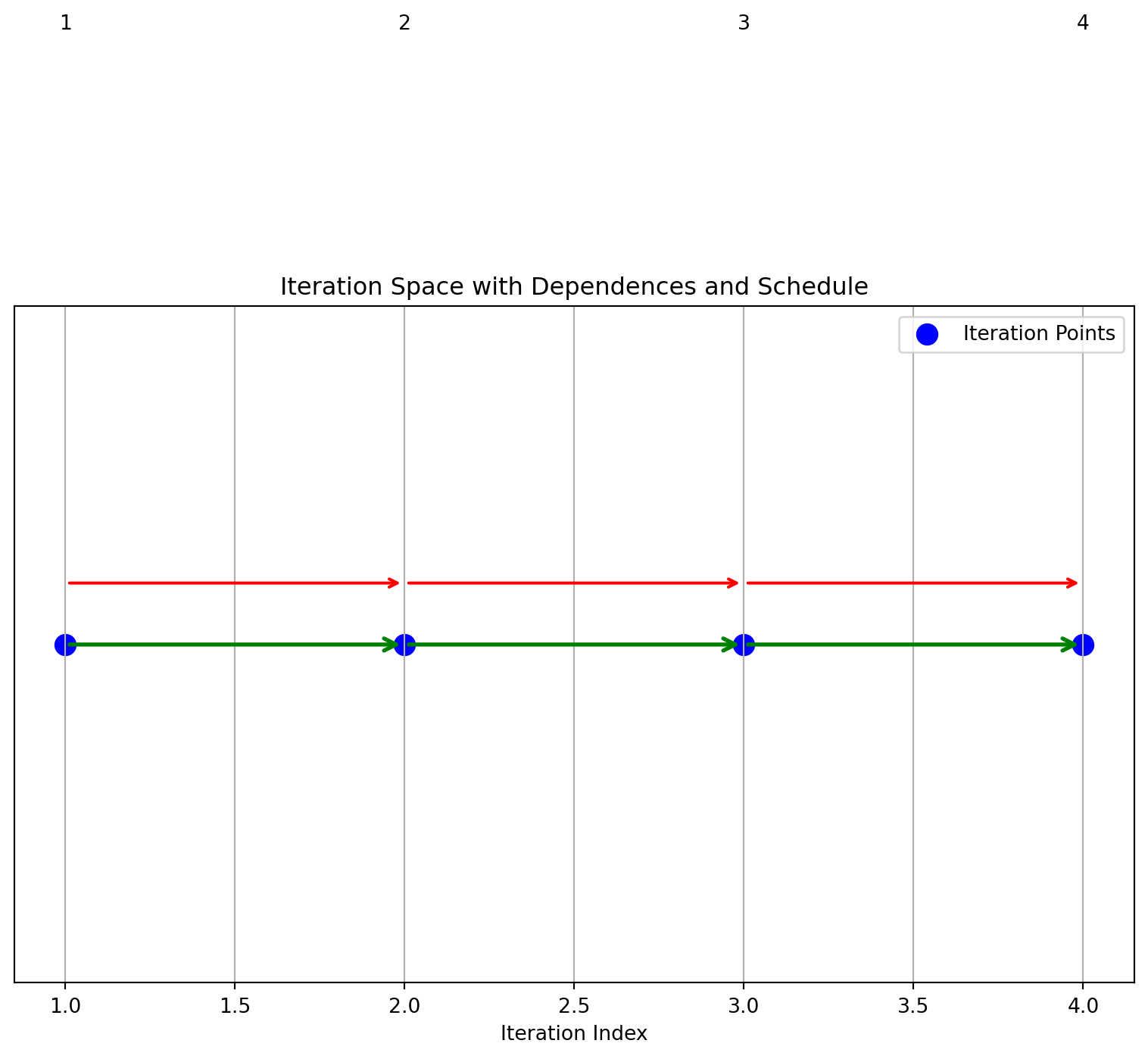
Many modern programs in fields like High-Performance Computing (HPC), GPU programming, scientific applications and machine learning are loop-intensive.
Traditional compiler techniques encounter several challenges in these contexts:

challenges

Complex Loop Dependencies:
- Dependencies can exist both within a loop and across multiple loops, limiting optimization potential.
Missed Parallelism:
- Insufficient analysis may prevent identification of potential parallel execution paths, underutilizing hardware capabilities.
Poor Data Locality:
- Inefficient usage of cache memory leads to performance bottlenecks.

Polyhedral methods address these challenges by providing a precise mathematical framework for analyzing and optimizing loop nests.

Challenges in Traditional Loop Optimization

for (i = 0; i < N; i++)  
  for (j = 0; j < N; j++)  
    A[i][j] = A[i-1][j] + A[i][j-1];

Iteration Dependencies
- $A[i][j]$ depends on $A[i-1][j]$ and $A[i][j-1]$
- Limits parallel execution due to data dependencies.
Performance Bottleneck
- Without optimization such as tiling, loop execution suffers from cache misses.

Improving Loop Performance by tiling

Benefits of Tiling

Improved Cache Access Patterns
- Reduces cache misses by increasing data locality.
Enhanced Parallelism
- Breaking dependencies across tiles can allow independent execution of tiles on different processors.

Example Tiling Transformation

Transform the inner loops by introducing tile sizes $T_i$ and $T_j$:

for (ii = 0; ii < N; ii += T_i)
  for (jj = 0; jj < N; jj += T_j)
    for (i = ii; i < min(ii + T_i, N); i++)
      for (j = jj; j < min(jj + T_j, N); j++)
        A[i][j] = A[i-1][j] + A[i][j-1];

Limitations of Polyhedral Methods

Affine Loops:
- Only applicable to loops with linear bounds and affine array accesses.
- Example: Bounds and accesses must be simple linear expressions of loop indices.
- Static Control Flow:
- Methods require loops without complex control flow such as recursion or unpredictable branches (virtual functions).

scops

Regions of code that can be handled in the polyhedral model are usually called Static Control Parts, abbreviated as SCoPs.

Usually, SCoPs may only contain regular control flow free of exceptions and other constructs that may provoke changes in control flow such as conditional expressions dependent on data (read from memory) or side effects of function calls.

loop free code can be a wrapped in for(i = 0; i < 1; i++){}

two kinds of problems

Polyhedral Analysis

Given a transformation. - Does a transformation preserve the loop’s semantics? - What is the resulting loop structure after transformation?

Polyhedral Scheduling

Find the “best” transformation that optimizes a property such as parallelism or data locality.

Advantages of Polyhedral Methods

Mathematical Rigor

Affine Constraints:
- Precisely model and manipulate loops, ensuring correctness.

Advanced Optimizations Enabled

Loop Tiling:
- Boosts data locality by breaking loops into smaller blocks.
Loop Fusion:
- Minimizes overhead and improves cache performance by combining adjacent loops.
Skewing and Parallelization:
- Addresses complex dependencies, allowing effective parallel execution.

Loop Execution

Statements and Instances

In loops, statements can execute multiple times.
Each execution of a statement is called an instance.
Polyhedral methods track these instances explicitly.

for i in [1, 2, 3, 4]:
  s: a[i] = 3  // Statement `s` executes four times (4 instances)

Program Representation

Statements and Index Sets
- Define what computations to perform.
- Specify the indices for which these computations are valid.
Schedule
- specifies the order in which the indices are executed.

Toy Example: Changing the Order of Iterations

Problem: Can we reverse this loop’s execution order?

for i = [1,2,3,4]
s:   a[i] = a[i-1]

Original schedule: i = 1, 2, 3, 4

Reversed schedule: i = 4, 3, 2, 1

Do these loops produce the same result?

for i = [1,2,3,4]               for i = [4,3,2,1]
s:   a[i] = a[i-1]               s:   a[i] = a[i-1]

Execution Trace and Data Access

Original Order	Reversed Order
Instance s(1): Reads a[0], Writes a[1]	Instance s(4): Reads a[3], Writes a[4]
Instance s(2): Reads a[1], Writes a[2]	Instance s(3): Reads a[2], Writes a[3]
Instance s(3): Reads a[2], Writes a[3]	Instance s(2): Reads a[1], Writes a[2]
Instance s(4): Reads a[3], Writes a[4]	Instance s(1): Reads a[0], Writes a[1]

data dependency

The data dependency arises from the use of $𝑎[𝑖−1]$ which has to be computed before $a[i]$

This kind of data dependency is called read after write or raw dependency

transformation

we propose a transformation $i \rightarrow 5 -i$ Does this transformation preserve all the dependencies?

a transformation is a change to the schedule

Schedules:

A schedule is a function:

\[s(\text{iteration}) = \text{execution order}(\text{time})\]

Example:

Original order: s(i) = i

Reversed order: s(i) = 5 - i

Producers must execute before consumers for the transformation to be valid.

schedule validity

not valid: if there is a pair $i$,$j$, $s[i]$ produces a value, $s[j]$ reads that value, and $s[j]$ is first in the new schedule

How do we find such a pair?

Visualization

Graphical Representation:
- Nodes represent statements with iteration index.
- Directed edges indicate data dependencies.
- Valid schedules respect edge directions.

forward order

iteration_space = [1,2,3,4]
dependences = [(1,2), (2,3), (3,4)]
schedule = [1,2,3,4]
draw_1d_iteration_space_with_dependence_graph(iteration_space, dependences, schedule)

Schedule:  [1, 2, 3, 4]

backward order

iteration_space = [1,2,3,4]
dependences = [(1,2), (2,3), (3,4)]
schedule= [4,3,2,1]
draw_1d_iteration_space_with_dependence_graph(iteration_space, dependences, schedule)

Schedule:  [4, 3, 2, 1]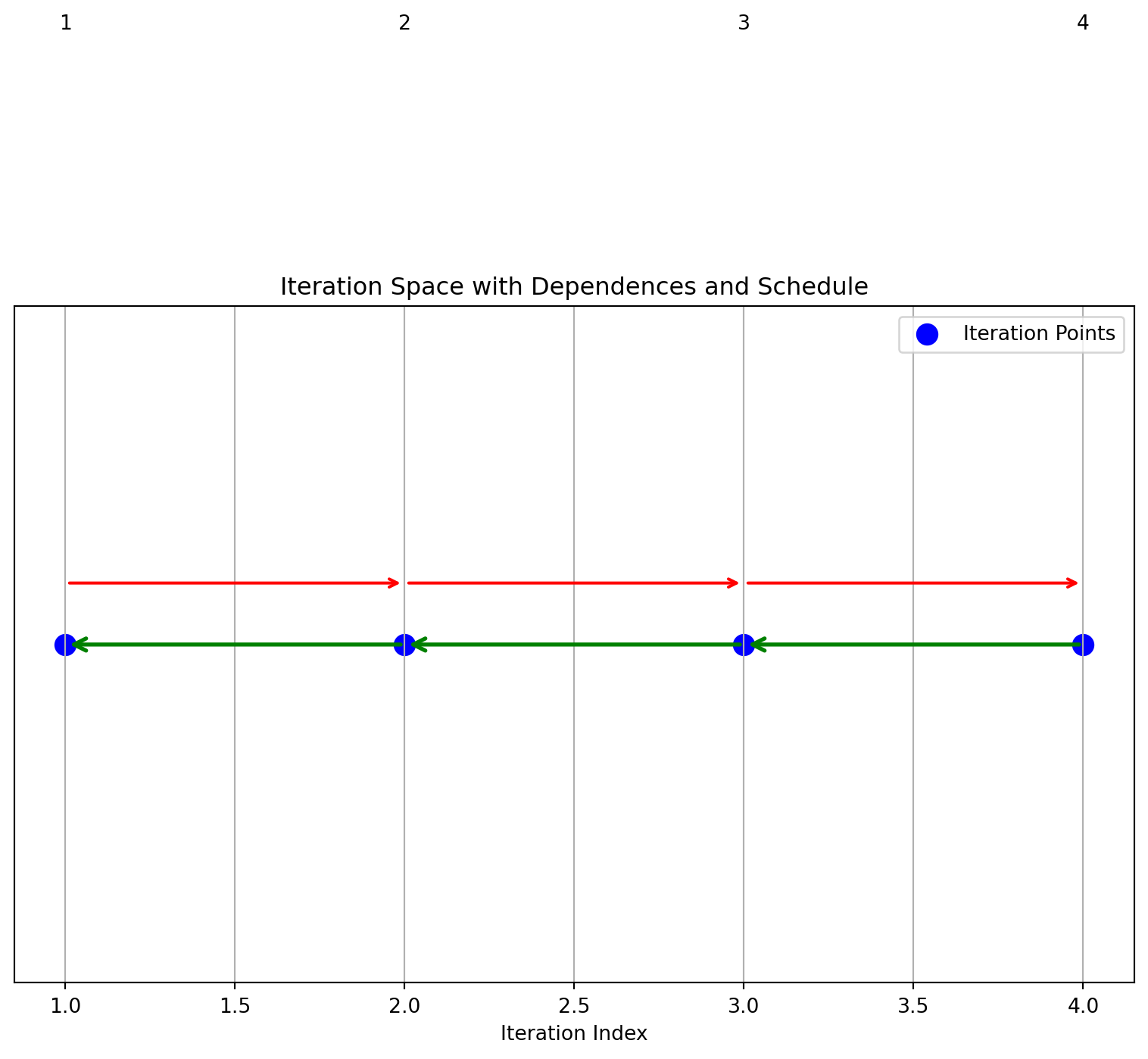

a schedule is not valid if the arrows go in different directions

more analytical check for valid

There are a number of tests for validity.

Mathematical Condition

Find $i, j$ where: \[\text{s}(i) < \text{s}(j) : i \text{ executes first}\]
- $i$ reads a value.
- $j$ writes that value.

One: an integer linear programming solver (ILP) to find an integer solution to the equations.

NP-hard but efficient solvers exist for many of the small cases found in programs

Two: check for a cycle in the graph

Analyzing Parallelism in Nested Loops

Code Example

for i in [1, 2, 3, 4]:
    for j in [1, 2, 3, 4]:
        a[i, j] = a[i, j-1] + a[i-1, j]

Can this Loop Nest be Executed in Parallel?

data dependence is a mapping:

$s(i) => s(i+1)$ from instance to instance

Horizontal Dependency:

Each iteration (i, j) depends on (i, j-1) (the value to the left in the same row).

1. For example, a[1, 2] = a[1, 1] + a[0, 2], which means a[1, 2] depends on the value of a[1, 1] from the same row. 
1. (1,1) -> (1,2)

Vertical Dependency:

Each iteration (i, j) depends on (i-1, j) (the value from the previous row in the same column).

1. For example, a[2, 1] = a[1, 1] + a[2, 0], meaning a[2, 1] depends on a[1, 1] from the row above
1. (1,1) -> (2,1)

Data Dependencies

True Dependency (Flow Dependency): When an instruction depends on the result of a previous instruction.
- Example: A = B + C followed by D = A + E
Anti Dependency: Occurs when an instruction requires a variable that will be overwritten by a subsequent instruction.
Output Dependency: When two instructions write to the same location, creating a dependency on the order of execution.

serial schedule

In a serial execution, iterations proceed row by row, strictly respecting both horizontal and vertical dependencies. This schedule respects all dependencies but executes sequentially, limiting parallelism.

visualization

iteration_space = [(1,1),(1,2),(1,3),(1,4),
                    (2,1),(2,2),(2,3),(2,4),
                    (3,1),(3,2),(3,3),(3,4),
                    (4,1),(4,2),(4,3),(4,4)]
dependences = []
for i in range(1, 5):
    for j in range(1, 5):
        if j > 1:  # Horizontal dependency
            dependences.append(( (i, j-1),(i, j)))
        if i > 1:  # Vertical dependency
            dependences.append(((i-1, j),(i, j) ))

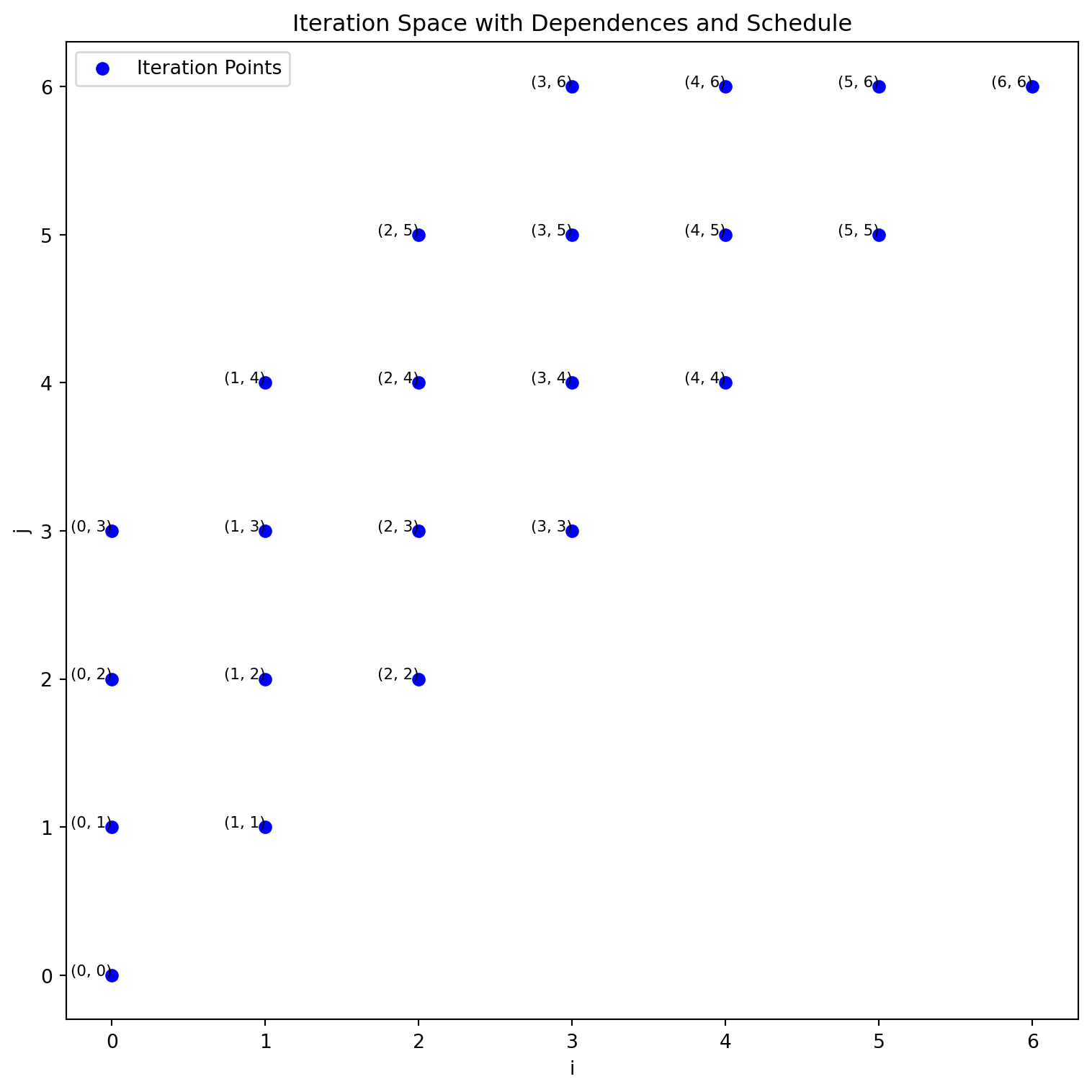
schedule = [(i, j) for i in range(1, 5) for j in range(1, 5)]
draw_2d_iteration_space_with_dependence_graph(iteration_space, dependences, schedule)

Schedule:  [(1, 1), (1, 2), (1, 3), (1, 4), (2, 1), (2, 2), (2, 3), (2, 4), (3, 1), (3, 2), (3, 3), (3, 4), (4, 1), (4, 2), (4, 3), (4, 4)]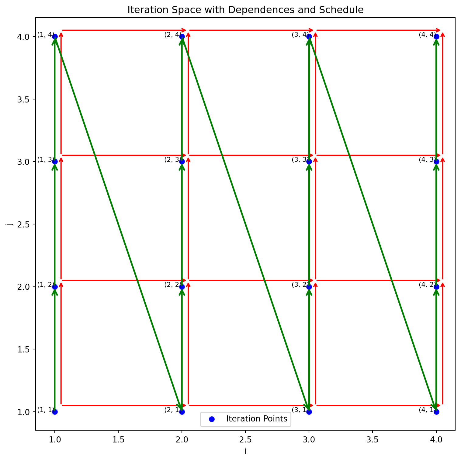

skewing the loops Parallel Schedule: Diagonal Parallelism

To maximize parallel execution in matrix computations, it’s crucial to identify and execute independent iterations simultaneously. One efficient strategy is Diagonal Parallelism:

Diagonal Organization: Process iterations by diagonals in the iteration space.
Diagonal Key: Defined as i + j (sum of indices).
Parallel Execution: Iterations with the same diagonal key (i + j constant) can be executed in parallel since they are independent.

Example: Diagonal Scheduling Code

# Organize the iteration space by diagonals
diagonals = {}
for (i, j) in iteration_space:
    diag_key = i + j  # Diagonal key: sum of indices
    if diag_key not in diagonals:
        diagonals[diag_key] = []
    diagonals[diag_key].append((i, j))

# Sort the diagonals by diagonal key
sorted_diagonals = sorted(diagonals.keys())

# Print the diagonal schedule
print("Diagonal Schedule:")
print(diagonals)

Diagonal Schedule:
{2: [(1, 1)], 3: [(1, 2), (2, 1)], 4: [(1, 3), (2, 2), (3, 1)], 5: [(1, 4), (2, 3), (3, 2), (4, 1)], 6: [(2, 4), (3, 3), (4, 2)], 7: [(3, 4), (4, 3)], 8: [(4, 4)]}

Visualizing the parallel schedule:

Schedule:  [(1, 1), (1, 2), (2, 1), (1, 3), (2, 2), (3, 1), (1, 4), (2, 3), (3, 2), (4, 1), (2, 4), (3, 3), (4, 2), (3, 4), (4, 3), (4, 4)]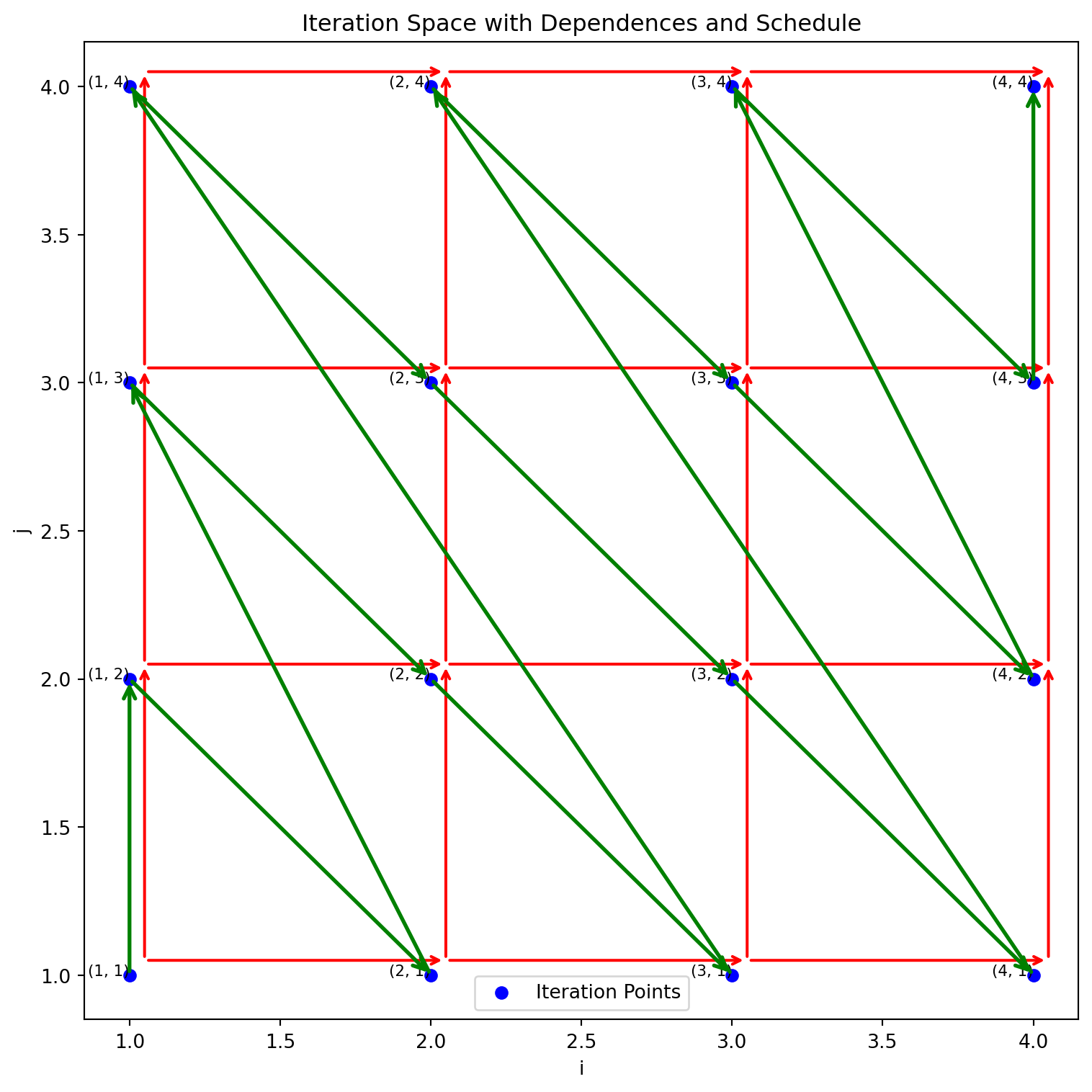

each diagonal line can run in parallel

Benefits of Diagonal Scheduling

Maximized Parallelism: All iterations of a diagonal can run concurrently.
Improved Cache Locality: Access patterns aligned to diagonals enhance data locality.
Scalability: Easily scalable on systems with symmetric multi-processing capabilities.

Definitions

Affine Functions of Loop Indexes

An affine function $f(\vec{v})$ is defined as:

\[f(\vec{v}) = M_f \vec{v} + \vec{f}_0\]

where:

$\vec{v}$ is a $d$-dimensional vector of loop indices:

\[\vec{v} = \begin{pmatrix} v_1 \\ \vdots \\ v_d \end{pmatrix}\]
$M_f$ is an integer matrix with $k$ rows and $d$ columns:

\[M_f \in \mathbb{Z}^{k \times d}\]
$\vec{f}_0$ is a $k$-dimensional integer translation vector:

\[\vec{f}_0 \in \mathbb{Z}^k\]

Note: All components are integers $\mathbb{Z}$.

affine functions

An affine function is a linear transformation followed by a translation. For example, each loop iteration $\vec{v}$ (e.g., $(i, j)$ in a 2D nested loop) can map iteration indices to dependence locations.

Loop Nest Types:

Perfect Loop Nest:

Definition: All statements are contained within the body of the innermost loop.
Example:

  for (int i = 0; i < N; i++) {
      for (int j = 0; j < N; j++) {
          a[i][j] = i + j;
      }
  }

Imperfect Loop Nest

Definition: There are statements located outside the innermost loop.
Example:

    for (int i = 0; i < N; i++) {
        b[i] = 0;
        for (int j = 0; j < N; j++) {
            a[i][j] += i * j;
        }
    }

Affine Loop Nest:

Characteristics:
- Loop bounds and array accesses are affine functions of outer loop variables and program parameters.
- Program parameters (e.g., $N$, $\beta$) are symbolic constants representing problem size.

domains in affine loops

if we look at the domain or index set of an affine loop nest we have a convex polyhedron

Understanding Polyhedrons and Polytopes

Polyhedron: Intersection of a finite number of planes.
Polytope: A bounded polyhedron.

Polyhedron Representation

Compact representation of a polyhedron: \[ \{\vec{x} \in \mathbb{Z}^n \mid A \vec{x} + \vec{b} \geq \vec{0}\} \]
- $A \in \mathbb{Z}^{m \times n}$
- $\vec{b} \in \mathbb{Z}^m$

Iteration Vector

The iteration vector $\vec{i}_S$ for a statement $S$ is a vector of loop indices from outermost to innermost. It represents a dynamic instance of $S$ in a loop nest.

Domain or Index Set

The domain (or index set) of a statement $S$ is the set of all its iteration vectors.

compiler notation

for (i=0 ; i<N ; i++)
    for (j=0 ; j<N ; j++) 
          s1: a(i, j) = a(i - 1, j) + 1;

just the domain

\[ \begin{aligned} i & \geq 0 \\ j & \geq 0 \\ -i+N-1 & \geq 0 \\ -j+N-1 & \geq 0 \end{aligned} \quad \quad \mathcal{D}^{S_{1}}:\left(\begin{array}{cccc} 1 & 0 & 0 & 0 \\ 0 & 1 & 0 & 0 \\ -1 & 0 & 1 & -1 \\ 0 & -1 & 1 & -1 \end{array}\right)\left(\begin{array}{c} i \\ j \\ N \\ 1 \end{array}\right) \geq 0 \]

We use a matrix and a vector to store a domain

adding in the dependence

we have ($i_\text{src}$, $j_\text{src}$), ($i_\text{dest}$, $j_\text{dest})$

both pairs are in the iteration space and $i_{\text{dest}} = i_{\text{src}} + 1, \quad j_{\text{dest}} = j_{\text{src}}$.

\[ \quad \quad \left(\begin{array}{cccc} 1 & 0 & 0 & 0 & 0 &0 \\ 0 & 1 & 0 & 0 & 0 & 0 \\ -1 & 0 &0&0& 1 & -1 \\ 0 & -1 &0& 0& 1 & -1 \\ 0 & 0 & 1 & 0 & 0 & 0 \\ 0 & 0 & 0 & 1 & 0 & 0 \\ -0 & 0 &-1&0& 1 & -1 \\ 0 & 0 &0& -1 & 1 & -1 \\ -1 & 0 & 1 &0 &0 &0 \\ 0 & -1 & 0 & 1 &0 &1 \end{array}\right)\left(\begin{array}{c} i_\text{src} \\ j_\text{src} \\ i_\text{dest}\\ j_\text{dest}\\ 1\\ N \end{array}\right) \geq 0 \]

Understanding Dependence in Matrix Computation

Original Code

for (i = 0; i < N; i++)
  for (j = 0; j < N; j++) 
     S1: A[i, j] = A[i, j] + u1[i] * v1[j] + u2[i] * v2[j];

for (k = 0; k < N; k++)
  for (l = 0; l < N; l++)
     S2: x[k] = x[k] + beta * A[l, k] * y[l];

Data Dependence: Occurs when multiple operations require reading from or writing to the same memory location.

matrix locations

Matrix Location Relation: A[i, j] potentially overlaps with A[l, k].

when

(0 i < N)
(0 j < N)
(0 k < N)
(0 l < N)
Dependence Conditions:
- If (i - l = 0), then the loop in S1 depends on the loop in S2.
- If (j - k = 0), there is potential write-after-read or read-after-write dependencies.

Loop Interchange Example

Original Loop Structure

for (i = 0; i < 9; i++)
  for (j = i; j < 7 && j < i + 4; j++)
     a[i,j] = 3;

Question

Can we reorder these loops?
Yes, we can reorder because there is no dependence.

Challenge: Determine the new loop bounds after interchange.

domain

loop bounds

original 

for (i = 0, i < 9; i++)
  for (j = i; j < 7 && j < i+4; j++)
     a[i,j] =  3

reordered 

for (j = 0; j <=6; j++)
 for (i = max(j-3,0); i <= j; i++)
   a[i,j] = 3

how do we get the reordered bounds?

Fourier-Motzkin Method for Variable Elimination

Purpose: Project a polyhedron onto a lower-dimensional space by eliminating variables from systems of linear inequalities.
Variable Elimination: Simplifies a system of linear inequalities by removing variables, reducing the dimensionality of the polyhedron while maintaining its feasibility.
Effective for systems in higher dimensions.

Steps of Fourier-Motzkin Elimination

Identify a Variable to Eliminate:
- Choose a variable (e.g., $i$) from the system to eliminate.
Rearrange Each Inequality:
- Solve each inequality for the chosen variable.
Eliminate the Variable:
- Combine pairs of inequalities to remove the chosen variable.
- Produce new inequalities in terms of the remaining variables.
Repeat the Process:
- Continue eliminating variables until only the desired ones remain.

back to this case

for (i = 0, i < 9; i++)
  for (j = i; j < 7 && j < i+4; j++)
     a[i,j] =  3

in the new version j will be the outer loop, so cannot use i in the bounds

Original Inequalities

$i \ge 0$
$i \le 8$ (since $i < 9$)
$i \le j$ (since loop starts at $j = i$)
$j \le 6$
$j \le i + 3$

Strategy: Eliminate `i` and Determine Bounds for `j`

To determine bounds for $j$, eliminate $i$:
- Find all constraints involving $i$: $L \le c_1 \cdot i$ and $c_2 \cdot i \le U$
- For each pair, derive: $c_2 \cdot L \le c_1 \cdot U$ along with constraints on $j$ only

Derived Constraints

Pair (1, 2): $0 \le 8$ — Ignore
Pair (1, 3): $0 \le j$
Pair (2, 5): $j - 3 \le j$ — Ignore
Pair (3, 5): $j - 3 \le 8$ ⇒ $j \le 11$ — Ignore
From inequality (4): $j \le 6$

Bounds for $j$: $0 \le j \le 6$

Solving for `i`

For the inner loop:
- $i \ge 0$ and $i \ge j - 3$ ⇒ $i \ge \max(0, j-3)$
- $i \le 8$ and $i \le j$ ⇒ ((8, j) = j), since $j \le 6$

Complexity of Fourier-Motzkin

Fourier-Motzkin elimination is computationally expensive, especially when the number of variables is large.

Worst-case complexity: The number of inequalities generated can grow exponentially with the number of variables, resulting in inefficient performance for high-dimensional systems. - Despite this, it is still a useful tool for small to medium-dimensional systems where the elimination process can be computationally feasible.

How much of a limitation is affine only

99% of hpc loops are affine: C. Bastoul, A. Cohen, S. Girbal, S. Sharma, and O. Temam. Putting polyhedral loop transformations to work. In LCPC, 2003.

over 95% of loops in deep learning are affine:

Norman P Jouppi, Cliff Young, Nishant Patil, David Patterson, Gaurav Agrawal, RaminderBajwa, Sarah Bates, Suresh Bhatia, Nan Boden, Al Borchers, et al. 2017. In-datacenter performance analysis of a tensor processing unit. In 2017 ACM/IEEE 44th Annual International Symposium on Computer Architecture (ISCA). IEEE, 1–12.

what about the ilp solver

ilp is np-complete so it is slow, but often tractable for problems with up to several hundred variables.

Some compiler writers feel that means poly methods can only do this for toy programs? - Is the complexity a barrier for real-world compiler applications?

Affine Functions

Only allow operations: addition, subtraction, multiplication by a constant.
Cannot multiply by unknowns or use quantifiers (e.g., ∀, ∃).
Can reformulate some problems but requires breaking them into simpler parts.

Multiple Dimensions and Data Dependencies

// Consider the following nested loops with data dependency in matrix A:
for (i = 1; i <= n; i++) {
    for (j = i; j <= n; j++) {
        // S: Data dependency on A[i-1][j] and A[i][j-1]
        A[i][j] = (A[i-1][j] + A[i][j-1]) * 0.5;
    }
}

The computation of $A[i][j]$ depends on $A[i-1][j]$ and $A[i][j-1]$, creating a pattern of data dependencies.

graph with tiles

Data Dependence for A[i][j] = (A[i-1][j] + A[i][j-1]) * 0.5
[((1, 1), (1, 2)), ((1, 2), (1, 3)), ((1, 3), (1, 4)), ((1, 4), (1, 5)), ((1, 5), (1, 6)), ((1, 6), (1, 7)), ((1, 7), (1, 8)), ((1, 2), (2, 2)), ((2, 1), (2, 2)), ((1, 3), (2, 3)), ((2, 2), (2, 3)), ((1, 4), (2, 4)), ((2, 3), (2, 4)), ((1, 5), (2, 5)), ((2, 4), (2, 5)), ((1, 6), (2, 6)), ((2, 5), (2, 6)), ((1, 7), (2, 7)), ((2, 6), (2, 7)), ((1, 8), (2, 8)), ((2, 7), (2, 8)), ((2, 3), (3, 3)), ((3, 2), (3, 3)), ((2, 4), (3, 4)), ((3, 3), (3, 4)), ((2, 5), (3, 5)), ((3, 4), (3, 5)), ((2, 6), (3, 6)), ((3, 5), (3, 6)), ((2, 7), (3, 7)), ((3, 6), (3, 7)), ((2, 8), (3, 8)), ((3, 7), (3, 8)), ((3, 4), (4, 4)), ((4, 3), (4, 4)), ((3, 5), (4, 5)), ((4, 4), (4, 5)), ((3, 6), (4, 6)), ((4, 5), (4, 6)), ((3, 7), (4, 7)), ((4, 6), (4, 7)), ((3, 8), (4, 8)), ((4, 7), (4, 8)), ((4, 5), (5, 5)), ((5, 4), (5, 5)), ((4, 6), (5, 6)), ((5, 5), (5, 6)), ((4, 7), (5, 7)), ((5, 6), (5, 7)), ((4, 8), (5, 8)), ((5, 7), (5, 8)), ((5, 6), (6, 6)), ((6, 5), (6, 6)), ((5, 7), (6, 7)), ((6, 6), (6, 7)), ((5, 8), (6, 8)), ((6, 7), (6, 8)), ((6, 7), (7, 7)), ((7, 6), (7, 7)), ((6, 8), (7, 8)), ((7, 7), (7, 8)), ((7, 8), (8, 8)), ((8, 7), (8, 8))]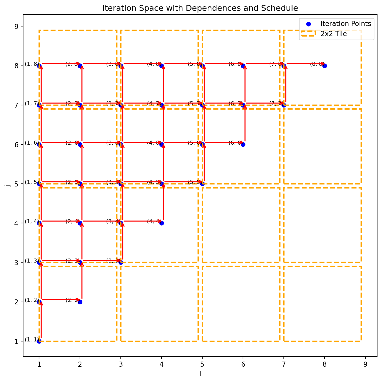

The schedule traverses the matrix in an upward direction for each column (j), moving left to right across columns (i).

adding tiles does not have a problem when dependence, but with-in each tile have to execute serially

Formalizing the Schedule: Lexicographic Ordering

Schedule Mapping: $s(i,j) \rightarrow (i,j)$
Statements as Vectors: Considered as ‘times’ (e.g., hours, minutes, seconds)

Understanding Lexicographic Ordering

\[(i,j) \gg (m,n) \iff i > m \lor (i = m \land j > n)\]

Compare elements from left to right.
Continue comparison on equal terms.
Lexicographic order generalizes alphabetical order (→).

Checking for loop interchange

for i in [1,2,3,4]                     for j in [1,2,3]
  for j in [1,2,3]                       for i in [1,2,3,4]
s:   a(i,j) = a(i-1,j+1)                   a(i,j) = a(i-1,j+1)

Original Schedule: $s(i, j) \rightarrow (i,j)$
After Interchange: $s(i,j) \rightarrow (j,i)$

data flow

        read write
s(1,1)  a(0,2)  a(1,1)
s(1,2)  a(0,3)  a(1,2)
s(1,3)  a(0,4)  a(1,3)
s(1,4)  a(0,5)  a(1,4)
s(2,1)  a(1,2)  a(2,1)   s(1,2)-> s(2,1)
s(2,2)  a(1,3)  a(2,2)   s(1,3)-> s(2.2)

\[ s(i,j) \rightarrow s(i+1, j-1) \]

constants:

Does there exist a statement s(i,j) and a statement $s(i',j')$ where in the new schedule $s(i',j')$ executes first and data flows backward in time \[ \begin{align*} (i', j') \gg (j,i) &\text{ $i',j'$ is first} \\ i' = 1+ i &\text{ data\ from \ i+1 to $i'$}\\ j' = -1 +j &\text{ data\ from \ j-1 to $j'$}\\ 1 \le i \le 4 \\ 1 \le j \le 3 \\ 1 \le i' \le 4 \\ 1 \le j' \leftrightarrows 3 \end{align*} \]

because of the lexicographic order we have two ilp problems one where $i'$ is greater then j, and one where $i'$ = j

solution

I ran it through:

https://online-optimizer.appspot.com

which gave me a solution:

s(4,2) reads s(3,3) but s(4,2) executes first

Classic transformations

loop reversal

transformation: [i] ==> [-i]

for (int c0 = 0; c0 < n; c0 += 1)
  S(c0);

for (int c0 = -n + 1; c0 <= 0; c0 += 1)
  S(-c0);

loop fusion

transformation: [0, i] -> [i,0]; [1, i] -> [i, 1]

{
  for (int c1 = 0; c1 <= n; c1 += 1)
    S(c1);
  for (int c1 = 0; c1 <= n; c1 += 1)
    T(c1);
}
for (int c0 = 0; c0 <= n; c0 += 1) {
  S(c0);
  T(c0);
}

loop fission

transformation: [i, 0] -> [0, i]; [i, 1] -> [1, i]

for (int c0 = 0; c0 <= n; c0 += 1) {
  S(c0);
  T(c0);
}
{
  for (int c1 = 0; c1 <= n; c1 += 1)
    S(c1);
  for (int c1 = 0; c1 <= n; c1 += 1)
    T(c1);
}

strip mining

transformation: [i] -> [floor(i/4), i % 4]

for (int c0 = 0; c0 <= 1023; c0 += 1)
  S(c0);

for (int c0 = 0; c0 <= 255; c0 += 1)
  for (int c1 = 0; c1 <= 3; c1 += 1)
    S(4 * c0 + c1);

loop tiling

transformation: [i,j] -> [floor(i/4), i % 4, floor(j/4), j % 4]

for (int c0 = 0; c0 <= 1023; c0 += 1)
  for (int c1 = 0; c1 <= 1023; c1 += 1)
    S(c0, c1);

for (int c0 = 0; c0 <= 255; c0 += 1)
  for (int c1 = 0; c1 <= 3; c1 += 1)
    for (int c2 = 0; c2 <= 255; c2 += 1)
      for (int c3 = 0; c3 <= 3; c3 += 1)
        S(4 * c0 + c1, 4 * c2 + c3);

finding transformations:

for i in [0, 1, 2, 3, 4, 5]:
    P:  a(i) = input(i) + 1
for j in [0, 1, 2, 3, 4, 5]:
    c:  b(j) = a(j) + 2

what transformation will give the best locality?

poly form

Each loop can be represented by its iteration space in a polyhedral form.

Loop 1: $𝑖 \in [0,1,2,3,5]$

Loop 2: $j \in [0,1,2,3,4,5]$

The dependencies between the two loops are: $p(i)$ must be computed before $c(i)$

define a new schedule

We introduce a schedule for each loop using affine transformations. (we can only handle affine transformations )

For the first loop: \[\theta_1(i) = \alpha_1 i + \beta_1\]

For the second loop: \[\theta_2(j) = \alpha_2 j + \beta_2\]

The goal is to reorder the iterations such that all dependencies are respected and memory locality is improved.

solving

We have to find four scalars

For all $i, j$ such that $p(i)$ sends data to $c(j)$, the following constraint holds:

\[\text{if } p(i) \to c(j), \quad \text{then } \theta_1(i) \leq \theta_2(j).\]

For all $0 \leq i \leq 5$ and $0 \leq j \leq 5$, and $i=j$ the following condition holds: \[\theta_1(i) \leq theta_2(j)\]

expanding this out

\[\alpha_1 i + \beta_1 \leq \alpha_2 j + \beta_2\]

looks bad- non-linear constraint since there is a product, and the foralls do not work with solvers

magic

We apply a theorem called the affine form of the Farkas lemma which turns this into a tractable problem

An affine form is non-negative over a polyhedron if and only if it can be be written as a non-negative combination of the constraints that form the polyhedron

forall $0 \le i \le 5$ and $0 \le j \le 5$ and $i = j$

such that $-\alpha_1 * i + \alpha_2 * j + (\beta_1 - \beta_2) \ge 0$ affine form

polyhedron

$i \ge 0$
$-i \ge -5$
$j \ge 0$
$-j \ge -5$
$j - i \ge 0$
$i=j \ge 0$

optimization problem

find a function that gives the locality

minimize w: $w \ge \alpha_2 * i + \beta_2 - \alpha_1 * j - \beta_1$

w is a bound in time between producer and consumer, how long the location needs to stay in the local memory

parallelism

we minimized the time between definition and use, for best locality, if we maximize that time we get the most parallel code

objectives

Since everything is affine it is hard to formulate a complex cost function

Other Formats